
Portfolio Optimization
Published:
Code for portfolio optimization using Modern Portfolio Theory.
Modern Portfolio Theory (MPT)
Modern Portfolio Theory (MPT), developed by Harry Markowitz in the 1950s, gives you a way to construct portfolios that maximize expected return for a given risk level (or equivalently, minimize risk for a given return). The core idea is that diversification across imperfectly correlated assets can reduce portfolio variance below the variance of any individual holding.
In this notebook we implement portfolio optimization from scratch and then use packages to automate it. We also compare different volatility estimation methods and see how they affect the results.
Equally-weighted portfolio
import yfinance as yf
import pandas_datareader.data as pdr
import seaborn as sns
import matplotlib.pyplot as plt
import numpy as np
import pandas as pd
import quantstats as qs

yf.pdr_override()

# Define a list of stock symbols belonging to tech sectors

stock_symbols = ["META", "TSLA", "X", "MSFT"]

# start date
start_date = '2018-01-01'
# end date
end_date = '2023-01-01'

# Fetch stock data along with sector information
prices_df = pdr.get_data_yahoo(stock_symbols,start_date,end_date)['Adj Close']


# assign equal weights to all assets
weights = np.array(len(stock_symbols) * [1 / len(stock_symbols)])


# returns
returns = prices_df.pct_change()
returns.dropna(inplace=True)


# portfolio returns into a dataframe
portfolio_returns = pd.Series(np.dot(returns,weights.T),index=returns.index)
[*********************100%%**********************] 4 of 4 completed
import logging
logging.getLogger('matplotlib.font_manager').setLevel(level=logging.CRITICAL)

# plot the portfolio performance
qs.plots.snapshot(portfolio_returns,title="Equal weight portfolio's performance",
grayscale=True)

plt.show()
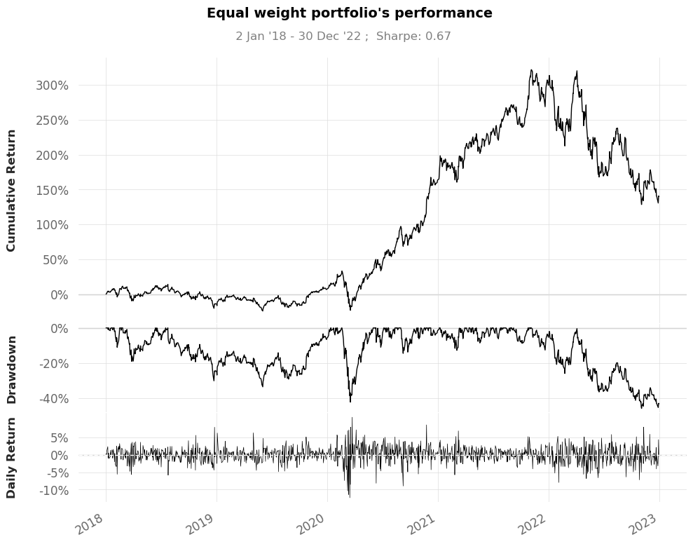
A drawdown refers to the peak-to-trough decline in the value of an investment or a trading account, typically expressed as a percentage. It represents the largest loss an investor or fund experiences before a new peak is reached.
# get the metric for the portfolio using bechmark SPY which follows S&P500
# for more detailed discussion on the metric, please refer to Portfolio_analysis.ipynb

qs.reports.metrics(portfolio_returns,benchmark="SPY",mode="basic",prepare_returns=False)
[*********************100%%**********************]  1 of 1 completed
                    Benchmark (SPY)    Strategy
------------------  -----------------  ----------
Start Period        2018-01-03         2018-01-03
End Period          2022-12-30         2022-12-30
Risk-Free Rate      0.0%               0.0%
Time in Market      100.0%             100.0%

Cumulative Return   41.39%             139.13%
CAGR﹪              4.91%              12.82%

Sharpe              0.43               0.66
Prob. Sharpe Ratio  82.94%             93.0%
Sortino             0.59               0.94
Sortino/√2          0.42               0.67
Omega               1.12               1.12

Max Drawdown        -34.1%             -45.84%
Longest DD Days     361                534

Gain/Pain Ratio     0.09               0.12
Gain/Pain (1M)      0.43               0.63

Payoff Ratio        0.89               0.92
Profit Factor       1.09               1.12
Common Sense Ratio  0.92               1.12
CPC Index           0.52               0.56
Tail Ratio          0.84               1.0
Outlier Win Ratio   5.26               2.75
Outlier Loss Ratio  5.08               2.82

MTD                 -6.19%             -12.17%
3M                  5.41%              -11.36%
6M                  0.55%              -12.72%
YTD                 -19.48%            -39.93%
1Y                  -19.91%            -40.54%
3Y (ann.)           3.8%               18.95%
5Y (ann.)           4.23%              11.89%
10Y (ann.)          4.91%              12.82%
All-time (ann.)     4.91%              12.82%

Avg. Drawdown       -2.41%             -5.76%
Avg. Drawdown Days  21                 32
Recovery Factor     1.36               2.62
Ulcer Index         0.09               0.17
Serenity Index      0.4                0.5
Portfolio variance is defined as:
\[\sigma_{port}^2 = weights^{T} \cdot Cov_{port} \cdot weights\]where \(Cov_{port}\) is the covariance matrix of the portfolio and \(weights\) is the vector of weights for each asset.
# variance matrix
var_yr = returns.cov() * 252

print(var_yr.shape,weights.T.shape,np.transpose(weights).shape)
# portfolio variance
port_var = weights.T@var_yr@weights

# portfolio volatility
port_vol = np.sqrt(port_var)

print(port_var, port_vol)
(4, 4) (4,) (4,)
0.13078861835379163 0.36164709089634833
In Modern Portfolio Theory (MPT), the goal is typically to either maximize the expected portfolio return for a given level of risk or minimize the portfolio risk for a given level of expected return. The optimization problem involves finding the weights of each asset in the portfolio that achieve these objectives. Here are the general formulas for the optimization problems in MPT:
Maximizing Expected Portfolio Return for a Given Level of Risk:
Objective: \(\text{Maximize} \quad \text{Expected Portfolio Return} = \sum_{i=1}^{n} w_i \cdot \text{Expected Return}_i\)
Subject to: \(\sum_{i=1}^{n} w_i = 1\) \(\text{Portfolio Variance} = \sum_{i=1}^{n} \sum_{j=1}^{n} w_i \cdot w_j \cdot \text{Covariance}_{ij} \leq \text{Target Risk}\)
Where:
- \(n\) is the number of assets in the portfolio.
- \(w_i\) is the weight of asset \(i\) in the portfolio.
- \(\text{Expected Return}_i\) is the expected return of asset \(i\).
- \(\text{Covariance}_{ij}\) is the covariance between the returns of assets \(i\) and \(j\).
- The constraint \(\sum_{i=1}^{n} w_i = 1\) ensures that the weights sum up to 1.
Minimizing Portfolio Risk for a Given Level of Expected Return:
Objective: \(\text{Minimize} \quad \text{Portfolio Variance} = \sum_{i=1}^{n} \sum_{j=1}^{n} w_i \cdot w_j \cdot \text{Covariance}_{ij}\)
Subject to: \(\sum_{i=1}^{n} w_i \cdot \text{Expected Return}_i \geq \text{Target Expected Return}\) \(\sum_{i=1}^{n} w_i = 1\)
Where:
- \(\text{Target Expected Return}\) is the desired level of expected return for the portfolio.
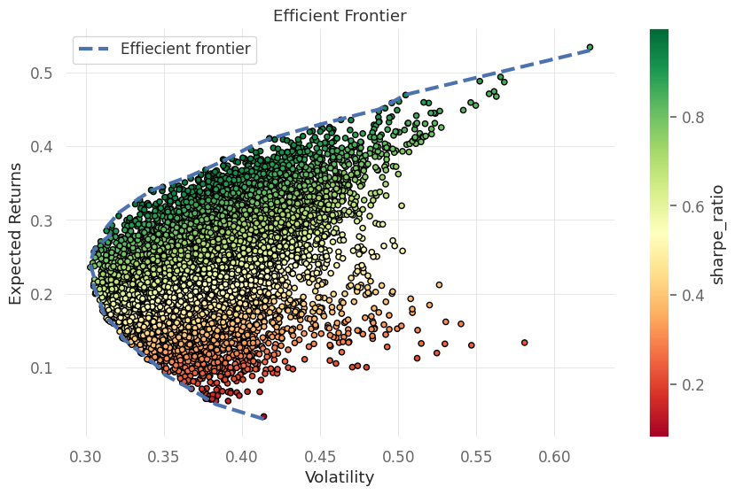
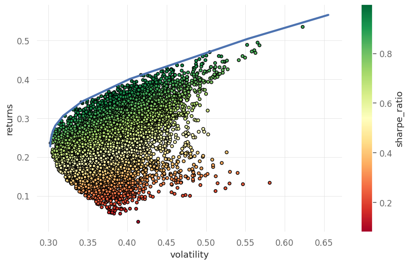
Efficient Frontier Using Monte Carlo
The efficient frontier is a set of optimal portfolios in the risk-return spectrum.
# Efficient frontier
import pandas as pd


mean_returns = returns.mean()
cov_matrix = returns.cov()
# Number of portfolios to simulate
nsim = 10000
# Risk free rate
risk_free_rate = 0.018

mean_returns = returns.mean() * 252
covariance_matrix = returns.cov() * 252

# generate random portfolio weights
np.random.seed(42)
weights = np.random.random(size=(nsim, len(stock_symbols)))
weights /=  np.sum(weights, axis=1)[:, np.newaxis]


port_retn = np.dot(weights, mean_returns)
port_vol = []
port_weights = []
# run simulation
for i in range(0, len(weights)):
    vol = np.sqrt(
        np.dot(weights[i].T, np.dot(covariance_matrix, weights[i]))
    )
    port_vol.append(vol)
    port_weights.append(weights[i])

# make an array
portf_vol = np.array(port_vol)

# get sharpe ratio
portf_sharpe_ratio = port_retn / portf_vol


# results df
results_df = pd.DataFrame(
    {"returns": port_retn,
    "volatility": portf_vol,
    "sharpe_ratio": portf_sharpe_ratio}
)

port_df = pd.DataFrame(port_weights,index=results_df.index,columns=stock_symbols)


# get maximum sharpe ratio
idx_maxsharpe = results_df["sharpe_ratio"].idxmax()
df_max_sharpe = results_df.iloc[idx_maxsharpe]
weight_max_sharpe = port_df.iloc[idx_maxsharpe]

# get minimum volatility
idx_minvol = results_df["volatility"].idxmin()
df_min_vol = results_df.iloc[idx_minvol]
weight_min_vol = port_df.iloc[idx_minvol]

npoints = 30
ef_rtn_list = []
ef_vol_list = []

# get range of returns
ef_retns = np.linspace(results_df["returns"].min(),results_df["returns"].max(),npoints)
# round the values
ef_retns = np.round(ef_retns, 2)

# actual returns
portf_rtns = np.round(port_retn, 2)

# for every return value find a minimum volatility
for rtn in ef_retns:
    if rtn in portf_rtns:
        ef_rtn_list.append(rtn)
        matched_ind = np.where(portf_rtns == rtn)
        ef_vol_list.append(np.min(portf_vol[matched_ind]))


# plot the results
fig, ax = plt.subplots()
results_df.plot(kind="scatter", x="volatility",
                    y="returns", c="sharpe_ratio",
                    cmap="RdYlGn", edgecolors="black",
                    ax=ax)

ax.set(xlabel="Volatility",ylabel="Expected Returns",title="Efficient Frontier")


ax.plot(ef_vol_list, ef_rtn_list, "b--",linewidth=3,label='Effiecient frontier')


ax.legend()
plt.show()
print("At maximum Sharpe Ratio\n")
print(f"Return:{df_max_sharpe['returns']}")
print(f"Volatility: {df_max_sharpe['volatility']}")
print(f"Portfolio: {weight_max_sharpe.to_dict()}")
print(f"Sharpe ratio: {df_max_sharpe['sharpe_ratio']}")
print("\n")
print("At Minimum risk\n")
print(f"Return:{df_min_vol['returns']}")
print(f"Volatility: {df_min_vol['volatility']}")
print(f"Portfolio: {weight_min_vol.to_dict()}")
print(f"Sharpe ratio: {df_min_vol['sharpe_ratio']}")
print("\n")
At maximum Sharpe Ratio

Return:0.34062078416847674
Volatility: 0.34168156067574446
Portfolio: {'META': 0.00021933368698373237, 'TSLA': 0.7269567018473118, 'X': 0.2574952867649712, 'MSFT': 0.015328677700733293}
Sharpe ratio: 0.996895423606794


At Minimum risk

Return:0.2357896874186083
Volatility: 0.3026424789381148
Portfolio: {'META': 0.0917403347472675, 'TSLA': 0.7961297432004478, 'X': 0.021304457291594758, 'MSFT': 0.09082546476068984}
Sharpe ratio: 0.7791030797987326
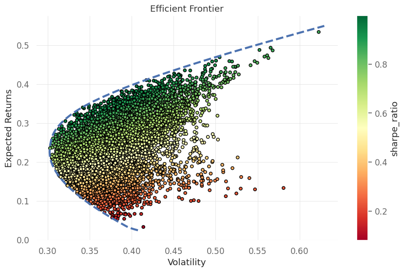
Efficient frontier using Scipy
In order to find the portfolio that gives highest returns for a given risk (volatility) or lowest risk (volatility) for a given return we can utilise numerical optimization. Optimization gives the best value of a function subjected to some boundary contraints affecting the target variable.
In the case of porfolio optimization we can express the equations as:
\[min (\omega^T \Sigma \omega)\]with constraints:
\begin{align} \omega^T \bold{I}=& b
\omega \geq& 0
\omega^{T}\mu =& \mu_p \end{align}
here \(\omega\) is the weight vector, \(\Sigma\) is the covariance matrix, \(\mu\) is the vector of returns with \(\mu_p\) is the expected portfolio return.
For a range of expected returns we find the optimal weights
Minimum risk
import numpy as np
import scipy.optimize as sco

# function to calculate portfolio return.
def portfolio_return(weights, asset_returns):
    return np.dot(weights, asset_returns)

# function to calculate portfolio volatility.
def portfolio_volatility(weights, covariance_matrix):
    return np.sqrt(np.dot(weights.T, np.dot(covariance_matrix, weights)))

# function to efficient portfolios along the efficient frontier.
def Efficient_frontier(asset_returns, covariance_matrix, target_returns):
    """
    Parameters:
    - asset_returns (array): Array of average returns for each asset.
    - covariance_matrix (array): Covariance matrix of asset returns.
    - target_returns (array): Array of target returns for which efficient portfolios are generated.
    """
    efficient_portfolios = []

    # Number of assets
    n_assets = len(asset_returns)

    # Define bounds for weights (between 0 and 1)
    bounds = tuple((0, 1) for _ in range(n_assets))

    # Initial guess for weights (equally weighted)
    weights0 = n_assets * [1. / n_assets, ]

    # Loop through target returns and find corresponding efficient portfolios
    for target_return in target_returns:
        # Constraints for optimization
        constraints = (
            {"type": "eq", "fun": lambda weights: portfolio_return(weights, asset_returns) - target_return},
            {"type": "eq", "fun": lambda weights: np.sum(weights) - 1}
        )

        # Optimize for minimum volatility
        result = sco.minimize(
            portfolio_volatility,
            weights0,
            args=(covariance_matrix,),
            method="SLSQP",
            constraints=constraints,
            bounds=bounds
        )

        # Save information about the efficient portfolio
        efficient_portfolios.append({
            'Return': target_return,
            'Volatility': result.fun,
            'Weights': result.x.tolist()
        })

    return efficient_portfolios


# define returns range
returns_range = np.linspace(0.025, 0.55, 400)

# covariance matrix
covariance_matrix = returns.cov() * 252

# asset returns
asset_returns = returns.mean() * 252

# run efficient frontier optimization
efficient_portfolios = Efficient_frontier(asset_returns, covariance_matrix, returns_range)

# volatility range
volatility_range = [p['Volatility'] for p in efficient_portfolios]


# plot efficient frontier

fig, ax = plt.subplots()

results_df.plot(kind="scatter", x="volatility",y="returns", c="sharpe_ratio",cmap="RdYlGn", edgecolors="black",ax=ax)

ax.plot(volatility_range, returns_range, "b--", linewidth=3)
ax.set(xlabel="Volatility",ylabel="Expected Returns",title="Efficient Frontier")
plt.show()
min_vol_ind = np.argmin(volatility_range)
min_vol_portf_rtn = returns_range[min_vol_ind]
min_vol_portf_vol = efficient_portfolios[min_vol_ind]["Volatility"]
min_vol_weights = efficient_portfolios[min_vol_ind]["Weights"]

min_vol_weights = dict(zip(stock_symbols, min_vol_weights))

print("At Minimum risk\n")
print(f"Return: {min_vol_portf_rtn}")

print(f"Volatility: {min_vol_portf_vol}")
print(f"Sharpe Ratio: {min_vol_portf_rtn / min_vol_portf_vol}")
print(f"weights: {min_vol_weights}")
print(f"Sharpe Ratio: {(min_vol_portf_rtn / min_vol_portf_vol)}")
At Minimum risk

Return: 0.2276315789473684
Volatility: 0.30210659990319516
Sharpe Ratio: 0.7534809865799325
weights: {'META': 0.0937157693026046, 'TSLA': 0.8067261730061059, 'X': 0.0, 'MSFT': 0.09955805769128928}
Sharpe Ratio: 0.7534809865799325
The minimum volatility portfolio is achieved by investing mostly in TESLA, Meta and Microsoft while not investing in X at all.
Maximum Sharpe Ratio
# define negative sharpe ratio for a optimization
def neg_sharpe(weight, avg_rtns, covariance_matrix, risk_free_rate):
    # calculate portfolio return and volatility
    port_ret = np.sum(avg_rtns * weight)
    port_vol = np.sqrt(np.dot(weight.T, np.dot(covariance_matrix, weight)))

    # get sharpe ratio
    port_sr = (
        (port_ret - risk_free_rate) / port_vol)

    return -port_sr

# we are searching for the portfolio with maximum sharpe ratio so we need to optimize for negative sharpe ratio

average_returns = returns.mean() * 252
covariance_matrix = returns.cov() * 252
# assume zero risk free rate
risk_free_rate = 0.


args = (average_returns,covariance_matrix,risk_free_rate)

# contraints
constraints = (
    {
        "type": "eq",
        "fun": lambda x: np.sum(x) - 1
    }
)

# bounds for weights
bounds = tuple((0, 1) for stock in range(len(stock_symbols)))

# initial guess
weight0 = np.array(len(stock_symbols) * [1. / len(stock_symbols)])

# minimize the function

max_sharpe = sco.minimize(neg_sharpe,
                                x0=weight0,
                                args=args,
                                method="SLSQP",
                                bounds=bounds,
                                constraints=constraints)

# make dictionary containing results
max_sharpe_port = {

    "returns": portfolio_return(max_sharpe.x,average_returns),
    "volatility": portfolio_volatility(max_sharpe.x,covariance_matrix),
    "sharpe_ratio": -max_sharpe.fun,
    "weights": max_sharpe.x.tolist()

}

# get weights df
max_sharpe_weights = dict(zip(stock_symbols, max_sharpe_port["weights"]))

print("At maximum sharpe ratio\n")
print(f"Return: {max_sharpe_port['returns']}")
print(f"Volatility: {max_sharpe_port['volatility']}")
print(f"Sharpe Ratio: {max_sharpe_port['sharpe_ratio']}")
print(f"weights: {max_sharpe_weights}")
At maximum sharpe ratio

Return: 0.3632417567223674
Volatility: 0.3612470733167341
Sharpe Ratio: 1.0055216596976673
weights: {'META': 0.0, 'TSLA': 0.6746528482243279, 'X': 0.32534715177567214, 'MSFT': 0.0}
The analysis indicates that most weight should be in TESLA and X with no allocation to META and Microsoft
Efficient frontier using convex optimization
Instead of optimizing the portfolio using mean-variance we can pose the problem in risk-adjusted retrun maximization. The problem then becomes:
\begin{align} max( \omega^T\mu -& \gamma \omega^T \Sigma \omega)
\omega^T\bold{I} =& 1
\omega \geq& 0 \end{align}
Here, \(\gamma \in [0,\infty)\) is risk aversion parameter. Higher value suggest more risk aversion.
This is a convex problem (quadratic objective, linear constraints), so any local minimum is the global minimum. We can solve it with cvxpy.
import cvxpy as cp

# setup the cvxpy variables
weights = cp.Variable(len(stock_symbols))

# risk aversion factor
gamma_para = cp.Parameter(nonneg=True)

# portfolio return
port_ret_cvx = mean_returns.values@weights

# portfolio volatility
port_vol_cvx = cp.quad_form(weights, covariance_matrix.values)

# define function
obj_fun = cp.Maximize(port_ret_cvx - gamma_para * port_vol_cvx)

# define problem and add constraints
prob = cp.Problem(obj_fun,[cp.sum(weights) == 1, weights >= 0])
# place holder for portfolio return, volatility and weights
port_ret_cvx_ef = []
port_vol_cvx_ef = []
weights_ef = []

# define gamma range
gamma_range = np.logspace(-3, 3, num=25)

# loop through gamma
for gamma in gamma_range:
    # set value of gamma
    gamma_para.value = gamma
    # solve problem
    prob.solve()
    # get portfolio return
    port_vol_cvx_ef.append(cp.sqrt(port_vol_cvx).value)
    # get portfolio volatility
    port_ret_cvx_ef.append(port_ret_cvx.value)
    # get portfolio weights
    weights_ef.append(weights.value)


# create dataframe for weights

weights_df = pd.DataFrame(weights_ef, index=np.round(gamma_range,3),columns=stock_symbols)
# plot the weight allocation for different gamma

fig,ax = plt.subplots(1,1)

weights_df.plot(kind='bar',ax=ax,stacked=True,title="Weights per gamma",xlabel="Gamma",ylabel="Weights")

plt.show()
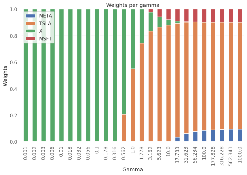
For low risk aversion the allocation is 100% to X but as the risk aversion increases the majority of allocation is in TESLA.
# plot efficient frontier
fig,ax = plt.subplots(1,1)
ax.plot(port_vol_cvx_ef, port_ret_cvx_ef, "b-", linewidth=3)

results_df.plot(kind="scatter", x="volatility",y="returns", c="sharpe_ratio",cmap="RdYlGn", edgecolors="black",ax=ax)
<Axes: xlabel='volatility', ylabel='returns'>
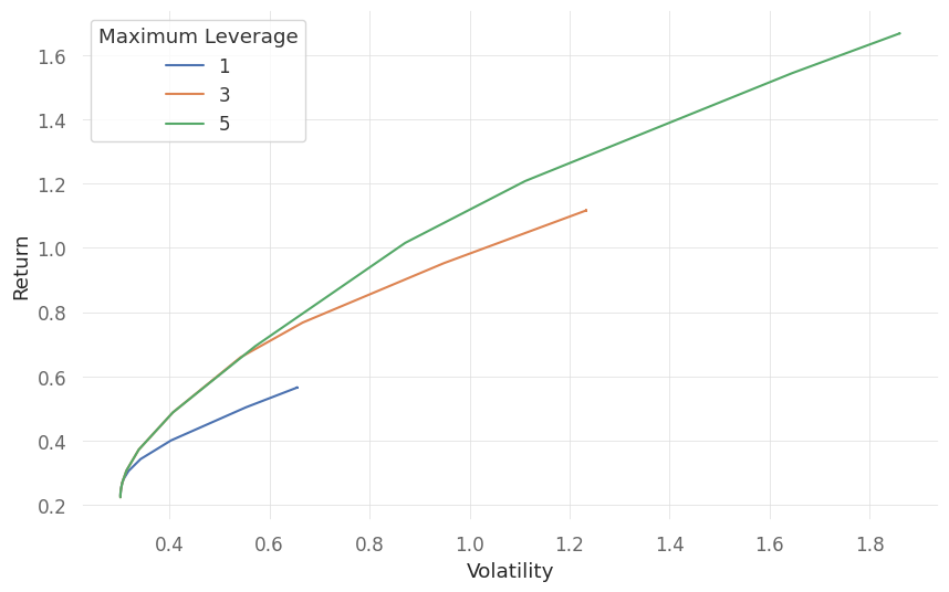
Maximum allowed Leverage
Leverage lets you borrow to invest more than your own capital. A leverage ratio of 2:1 means for every $1 of your capital, you can invest $2 total. Higher leverage amplifies both gains and losses.
We can add a leverage constraint by bounding the L1 norm of the weight vector:
# define maximum leverage parameter
max_leverage = cp.Parameter()

# define problem with leverage
prob_with_l = cp.Problem(obj_fun,
    [cp.sum(weights) == 1,
    cp.norm(weights, 1) <= max_leverage])


# range of leverage
lev_range = [1,3,5]

N = len(gamma_range)
# place holder for portfolio return, volatility and weights
portfolio_return = np.zeros((N,len(lev_range)))
portfolio_volatility = np.zeros((N,len(lev_range)))
portfolio_weights = np.zeros((len(lev_range),N,len(stock_symbols)))
# loop through leverage and gamma
# record the results in the placeholders

for l,lev in enumerate(lev_range):
    for g in range(N):
        # set values of variables
        max_leverage.value = lev
        gamma_para.value = gamma_range[g]
        # solve the equations
        prob_with_l.solve()
        # fill the values in place holders
        portfolio_return[g,l] = port_ret_cvx.value
        portfolio_volatility[g,l] = cp.sqrt(port_vol_cvx).value
        portfolio_weights[l,g,:] = weights.value
# plot the weights for different gamma

fig,ax = plt.subplots(1,1)
ax.set_xlabel(r'Volatility')
ax.set_ylabel(r'Return')

for k,lev in enumerate(lev_range):
    ax.plot(portfolio_volatility[:,k], portfolio_return[:,k], label=f"{lev}")

ax.legend(title="Maximum Leverage")
plt.show()
# plot the allocation for different allocation for different leverage and gamma

fig,axes = plt.subplots(len(lev_range),1,sharex=True)

for axi in range(len(axes)):

    weights_df = pd.DataFrame(portfolio_weights[axi], index=np.round(gamma_range,3),columns=stock_symbols)

    weights_df.plot(kind='bar',ax=axes[axi],stacked=True,xlabel="Gamma",ylabel=f"max lev = {lev_range[axi]} \n Weights",legend=None)

axes[0].legend(bbox_to_anchor=(1, 1))
axes[0].set_title("Weights per risk aversion")

plt.show()
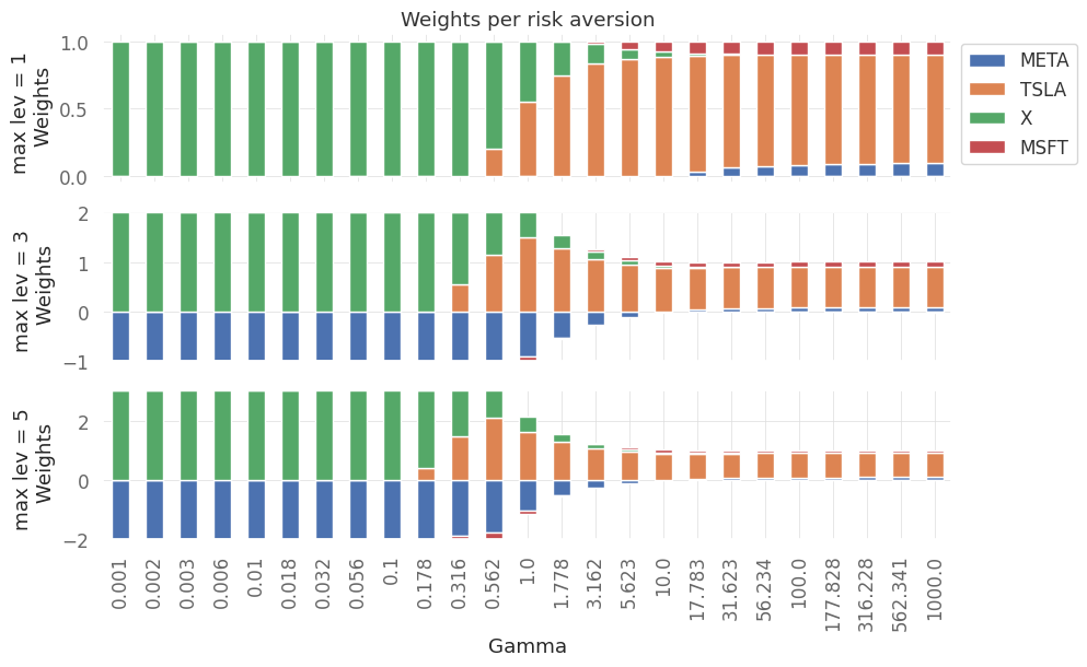
we note that with an increase in risk aversion, all cases converge to a similar allocation for all levels of the leverage.
Traditional optimization methods depend on inverting covariance matrix. They are also unstable. More correlated assets lead to need of more diversification and which leads to more errors in calculation of portfolio weights.
Hierarchical Risk Parity
Hierarchical Risk Parity (HRP), introduced by Marcos Lopez de Prado, takes a different approach from mean-variance optimization. Instead of inverting the covariance matrix (which is unstable when assets are correlated), it uses hierarchical clustering to group similar assets and then allocates inversely proportional to each cluster’s variance.
The steps:
- Dendrogram construction — cluster assets by pairwise correlation into a tree structure.
- Recursive bisection — split the tree into sub-clusters at each level.
- Inverse variance weighting — within each cluster, weight assets inversely by their variance (lower-risk assets get more weight).
- Bottom-up allocation — repeat at each level of the hierarchy, then combine into final portfolio weights.
The main advantage over mean-variance: HRP doesn’t require inverting the covariance matrix, so it’s more stable when you have many correlated assets or limited data.
import yfinance as yf
import pandas_datareader.data as pdr
import seaborn as sns
import matplotlib.pyplot as plt
import numpy as np
import pandas as pd
import quantstats as qs

yf.pdr_override()
from pypfopt.expected_returns import returns_from_prices
from pypfopt.hierarchical_portfolio import HRPOpt
from pypfopt.discrete_allocation import DiscreteAllocation, get_latest_prices
from pypfopt import plotting
# Define a list of stock symbols

stocks = {'Apple Inc.': 'AAPL',
'Microsoft Corporation': 'MSFT',
'Amazon.com Inc.': 'AMZN',
'Alphabet Inc.': 'GOOGL',
'Meta Platforms, Inc.': 'META',
'Tesla, Inc.': 'TSLA',
'Johnson & Johnson': 'JNJ',
'JPMorgan Chase & Co.': 'JPM',
'Visa Inc.': 'V',
'Procter & Gamble Co.': 'PG',
'NVIDIA Corporation': 'NVDA',
'Mastercard Incorporated': 'MA',
'The Walt Disney Company': 'DIS',
'Salesforce.com Inc.': 'CRM'

}

stock_symbols = list(stocks.values())

# start date
start_date = '2018-01-01'
# end date
end_date = '2023-01-01'

stock_data = pdr.get_data_yahoo(stock_symbols,start_date,end_date)['Adj Close']

# returns
returns_df = returns_from_prices(stock_data)
[*********************100%%**********************] 14 of 14 completed
# Optimize using Hierarchical Risk Parity
hrp = HRPOpt(returns=returns_df)
hrp.optimize()

# get weights
weights = hrp.clean_weights()

print(weights)
OrderedDict([('AAPL', 0.05942), ('AMZN', 0.04517), ('CRM', 0.06996), ('DIS', 0.0784), ('GOOGL', 0.06652), ('JNJ', 0.16991), ('JPM', 0.08137), ('MA', 0.05232), ('META', 0.03086), ('MSFT', 0.06809), ('NVDA', 0.02474), ('PG', 0.15484), ('TSLA', 0.03146), ('V', 0.06692)])
# get portfolio performance
hrp.portfolio_performance(verbose=True, risk_free_rate=0);
Expected annual return: 16.1%
Annual volatility: 22.4%
Sharpe Ratio: 0.72
# plot the heirarchical clustering

fig,ax = plt.subplots()

ax.set_title("Dendogram for clusters")

plotting.plot_dendrogram(hrp, color_threshold=0, ax=ax, above_threshold_color='grey')

plt.show()
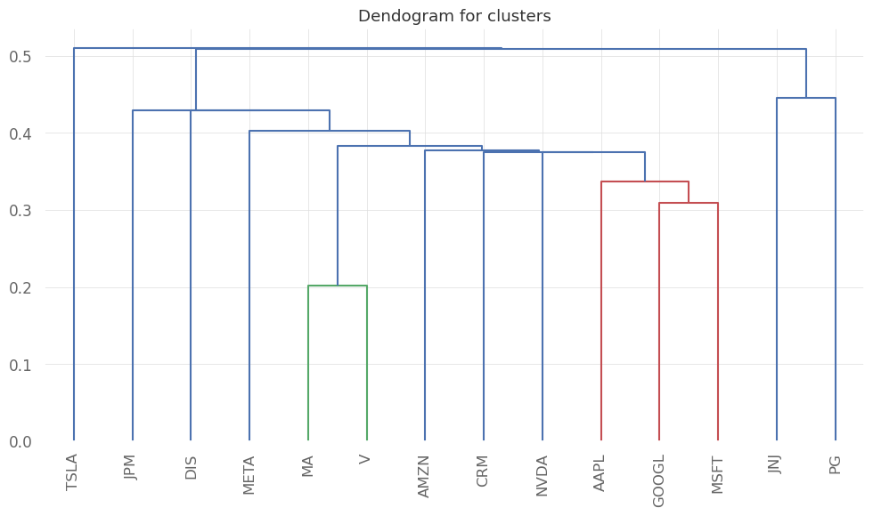
We see that similar companies are clustered together (eg. Visa and Mastercard or GOOGLE, Microsoft and Apple). So in order to diversify, we can choose companies belonging to different clusters.
We can also find the allocation for each company for a total amount of money we wish to invest.
# get current prices and allocate 100,000 USD
latest_prices = get_latest_prices(stock_data)

# find allocation based on weights using hrp
allocation_finder = DiscreteAllocation(weights,
        latest_prices,
        total_portfolio_value=100000)

# get portolio
allocation, leftover = allocation_finder.lp_portfolio()


for stock in stocks.keys():
        if stocks[stock] in allocation.keys():
                print(f"{stock}: {allocation[stocks[stock]]}")

print(f"Leftover: {leftover}")
Apple Inc.: 46
Microsoft Corporation: 29
Amazon.com Inc.: 54
Alphabet Inc.: 75
Meta Platforms, Inc.: 26
Tesla, Inc.: 26
Johnson & Johnson: 99
JPMorgan Chase & Co.: 62
Visa Inc.: 32
Procter & Gamble Co.: 105
NVIDIA Corporation: 17
Mastercard Incorporated: 15
The Walt Disney Company: 90
Salesforce.com Inc.: 53
Leftover: 1.369749858728028
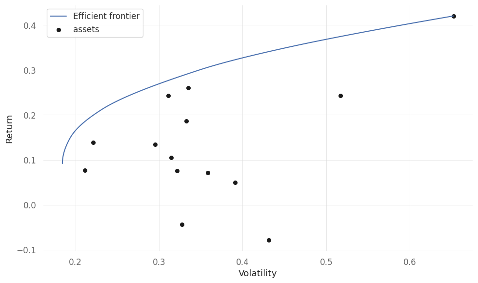
Efficient Forntier using PyPortfolioOpt
Sample covariance matrices get noisy when you have few observations relative to the number of assets. Ledoit-Wolf shrinkage addresses this by blending the sample covariance with a structured target (typically a scaled identity matrix), reducing estimation error.
from pypfopt.expected_returns import mean_historical_return
from pypfopt.risk_models import CovarianceShrinkage
from pypfopt.efficient_frontier import EfficientFrontier
from pypfopt.plotting import plot_efficient_frontier


# get mean and variance of returns
mu = mean_historical_return(stock_data, frequency=252)
covariance_matrix = CovarianceShrinkage(stock_data).ledoit_wolf()

# calculate the efficient frontier
EF = EfficientFrontier(mu, covariance_matrix)
# plot the EF
fig,ax = plt.subplots(1,1)

plot_efficient_frontier(EF, ax=ax, show_assets=True)

plt.show()
/home/ankitsingh/miniconda3/envs/DS/lib/python3.11/site-packages/cvxpy/reductions/solvers/solving_chain.py:336: FutureWarning:
    Your problem is being solved with the ECOS solver by default. Starting in
    CVXPY 1.5.0, Clarabel will be used as the default solver instead. To continue
    using ECOS, specify the ECOS solver explicitly using the ``solver=cp.ECOS``
    argument to the ``problem.solve`` method.

  warnings.warn(ECOS_DEPRECATION_MSG, FutureWarning)
# get weights for highest sharpe ratio
EF = EfficientFrontier(mu, covariance_matrix)
weights_ms = EF.max_sharpe()

# get weights for minimum volatility
EF = EfficientFrontier(mu, covariance_matrix)
weights_mv = EF.min_volatility()

# print weights
print("At maximum sharpe ratio\n")
for stock in stocks.keys():
        if stocks[stock] in weights_ms.keys():
                print(f"{stock}: {weights_ms[stocks[stock]]}")

print("\nAt minimum volatility\n")
for stock in stocks.keys():
        if stocks[stock] in weights_mv.keys():
                print(f"{stock}: {weights_mv[stocks[stock]]}")
At maximum sharpe ratio

Apple Inc.: 0.245191828703573
Microsoft Corporation: 0.223290432799307
Amazon.com Inc.: 0.0
Alphabet Inc.: 0.0
Meta Platforms, Inc.: 0.0
Tesla, Inc.: 0.1619657168958174
Johnson & Johnson: 0.0
JPMorgan Chase & Co.: 0.0
Visa Inc.: 0.0
Procter & Gamble Co.: 0.3695520216013028
NVIDIA Corporation: 0.0
Mastercard Incorporated: 0.0
The Walt Disney Company: 0.0
Salesforce.com Inc.: 0.0

At minimum volatility

Apple Inc.: 0.0
Microsoft Corporation: 0.0
Amazon.com Inc.: 0.0959515427915488
Alphabet Inc.: 0.0041594590053027
Meta Platforms, Inc.: 0.0
Tesla, Inc.: 0.0054829509292488
Johnson & Johnson: 0.4440479006669384
JPMorgan Chase & Co.: 0.0288517492601816
Visa Inc.: 0.0
Procter & Gamble Co.: 0.3507875353775004
NVIDIA Corporation: 0.0
Mastercard Incorporated: 0.0
The Walt Disney Company: 0.0707188619692793
Salesforce.com Inc.: 0.0