Time series analysis
Published:
We will discuss the time series analysis using finance data. The techniques like Moving Average (MA) , Autoregressive (AR) and Autoregressive Integrated Moving Average Model (ARIMA) will be dicussed. For modelling the time series we will be using the statsmodel library for the data acquired using Yahoo finance api.
Lets begin by importing the data of Microsoft for the years 2019-2021.
import yfinance as yfin
import numpy as np
import pandas as pd
import pandas_datareader.data as pdr
import statsmodels.api as sm
from statsmodels.tsa.seasonal import seasonal_decompose
from statsmodels.tsa.stattools import adfuller
from scipy import stats
import warnings

warnings.filterwarnings("ignore")

yfin.pdr_override()

# List of stock symbols
ticker = 'MSFT'

# Set the date range for the historical data
start_date = '2019-1-1'
end_date = '2021-1-1'
# Download historical stock data for each stock

stock = pdr.get_data_yahoo(ticker, start_date, end_date,interval='1d').Close


# choose data over 2 years
start_date = '2019-1-1'
end_date = '2021-1-1'

# get the data with 1d interval
stocks = pdr.get_data_yahoo(ticker, start_date, end_date,interval='1d').Close
stocks.dropna(inplace=True)
returns = stocks.pct_change()
returns.dropna(inplace=True)
stat_test = adfuller(returns.dropna())[0:2]
print(f"The test statistic and p-value of ADF test are {stat_test}")
if stat_test[1] < 0.05:
    print("The data is stationary")
else:
    print("The data is not stationary")

# split the data into train and test
split = int(len(returns.values) * 0.90)

price_train = stocks.iloc[:split+1]
price_test = stocks.iloc[split:]
return_train = returns.iloc[:split]
return_test = returns.iloc[split:]
print(return_test.shape,return_train.shape,price_test.shape,price_train.shape,stock.shape)
[*********************100%%**********************]  1 of 1 completed
[*********************100%%**********************]  1 of 1 completed
The test statistic and p-value of ADF test are (-7.212097179922102, 2.2211435488651752e-10)
The data is stationary
(51,) (453,) (52,) (454,) (505,)
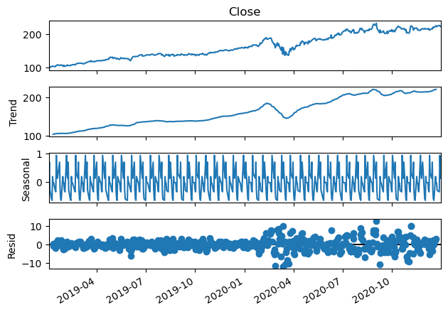
Lets quickly use the statsmodel to decompise the trend and seasonality in the data.
# Plot  the components of a time series by
# seasonal_decompose function from statsmodels
import matplotlib.pyplot as plt

seasonal_decompose(stock, period=12).plot()
plt.gcf().autofmt_xdate()
plt.show()
ACF and PCF
Auto-correlation functions (ACF) show the correlation between the same series with different lags. With h being the lag:
\[ρ(h) = \frac{Cov(X_t , X_{t−h} )}{Var(X_t )}\]The coefficients help in deciding the q in MA(q) models.
Partial ACF (PACF) gives information on correlation between current value of a time series and its lagged values controlling for the other correlations.
\[ρ(h) = \frac{Cov(X_t ,X_{t−h} |X_{t−1} ,X_{t−2} ...X_{t−h−1})}{ \sqrt{Var(X_t |X_{t−1} ,X_{t−2} ,...,X_{t−h−1} )Var(X_{t−h} |X_{t−1} ,X_{t−2} ,...,X_{t−h−1} )}}\]The coefficients help in deciding the p in AR(p) models.
sm.graphics.tsa.plot_acf(stock,lags=70)
plt.show()
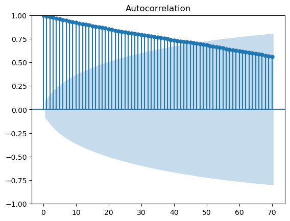
It shows that there is strong dependence between the current value and lagged values of stock data as the coefficients of autocorrelation decay slowly.
sm.graphics.tsa.plot_pacf(stock, lags=24)
plt.show()
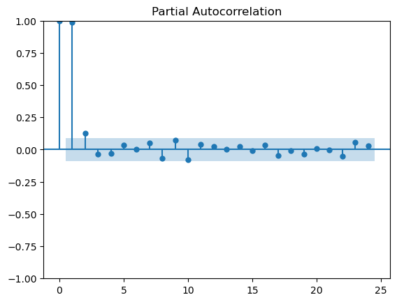
Lines above the confidence intervals are considered significant. We see the model with lag of 2 coefficient is enough to model the variations.
Time Series modeling
Moving Average (MA)
Moving average can be considered as smoothing model as it tends to take into account the lag values of residual.
For \(\alpha \ne 0\), MA(q) can be written as:
\[X_t = \epsilon_t + \alpha_1 \epsilon_{t−1} + \alpha_2 \epsilon_{t−2} ... + \alpha_q \epsilon_{t−q}\]
def ts_plots(data,lags):
    mosaic = """
    AA
    BC
    """
    fig = plt.figure(figsize=(8,8))
    ax = fig.subplot_mosaic(mosaic)
    ax['A'].plot(data)
    sm.graphics.tsa.plot_acf(returns.dropna(),ax=ax['B'],lags=lags)
    sm.graphics.tsa.plot_pacf(returns.dropna(),ax=ax['C'],lags=lags)

    fig.subplots_adjust()

ts_plots(returns,lags=30)
plt.show()
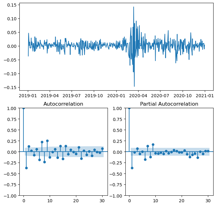
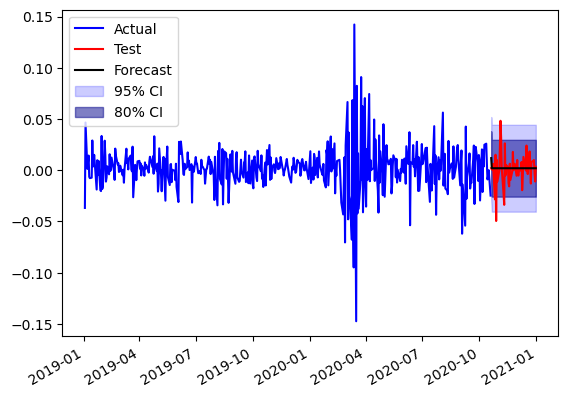
Peaks at 1 in ACF, we choose them order for MA i.e. MA(1) Model
from statsmodels.tsa.arima.model import ARIMA

modelMA = ARIMA(return_train, order=(0, 0, 1)).fit()

forecast = modelMA.get_forecast(steps=len(return_test))

conf_int95 = forecast.conf_int(alpha=0.05)
conf_int80 = forecast.conf_int(alpha=0.2)


fig,ax = plt.subplots()
ax.plot(return_train.index,return_train.values,color='b',label='Actual')
ax.plot(return_test.index,return_test.values,color='r',label='Test')
ax.plot(return_test.index,forecast.predicted_mean,color='k',label='Forecast')
ax.fill_between(return_test.index,conf_int95['lower Close'],conf_int95['upper Close'],alpha=0.2,color='b',label='95% CI')
ax.fill_between(return_test.index,conf_int80['lower Close'],conf_int80['upper Close'],alpha=0.5,color='darkblue',label='80% CI')

ax.legend(loc=2)
plt.gcf().autofmt_xdate()
# inspect residuals
modelMA.plot_diagnostics(figsize=(6,6))
plt.show()
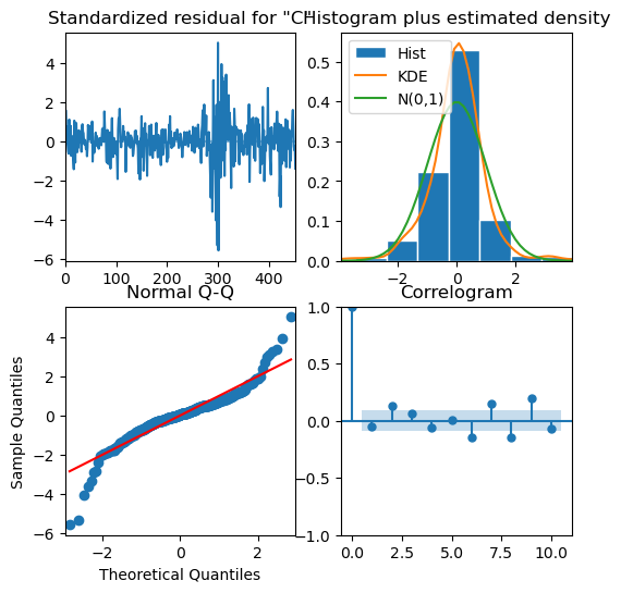
Residuals are white noise therefore, good fit
Transform back to prices
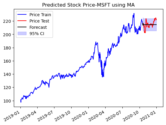
# use 95% confidence interval from above to return price forcasts and confidence intervals
pf=[]
pf.append(price_train[-1])
confd = []
confd.append(price_train[-1])
confu = []
confu.append(price_train[-1])

for ret,dn,up in zip(forecast.predicted_mean.values,conf_int95['lower Close'].values,conf_int95['upper Close'].values):
    new_price = price_train[-1] * (1 + ret)
    confu.append(price_train[-1] * (1 + up))
    confd.append(price_train[-1] * (1 + dn))

    pf.append(new_price)

fig,ax = plt.subplots()
ax.plot(price_train.index,price_train.values,color='b',label='Price Train')
ax.plot(price_test.index,price_test.values,color='r',label='Price Test')
ax.plot(price_test.index,pf,color='k',label='Forecast')
ax.fill_between(price_test.index,confd,confu,alpha=0.2,color='b',label='95% CI')
ax.set_title(f'Predicted Stock Price-{ticker} using MA')
ax.legend()
plt.gcf().autofmt_xdate()
conf_int80['lower Close'].iloc[i]
-0.025608780730429798
sm.stats.durbin_watson(modelMA.resid.values)
2.021053921541334
Short-term moving average tends to more reactive to daily activity and long MA captures the global trend, But still the model is not able to capture the trends
Autoregressive Model
Idea is the current value is regressed over its own lag values in this model. Forcast the current value of time series \(X_{t}\):
\[X_t = c + \alpha_1 X_{t−1} + \alpha_2 X_{t−2} ... + \alpha_p X_{t−p} + \epsilon_t\]We see a peak in the PCAF of data at p=1
from statsmodels.tsa.arima.model import ARIMA

modelMA = ARIMA(return_train, order=(1, 0, 0)).fit()

forecast = modelMA.get_forecast(steps=len(return_test))

conf_int95 = forecast.conf_int(alpha=0.05)
conf_int80 = forecast.conf_int(alpha=0.2)


fig,ax = plt.subplots()
ax.plot(return_train.index,return_train.values,color='b',label='Actual')
ax.plot(return_test.index,return_test.values,color='r',label='Test')
ax.plot(return_test.index,forecast.predicted_mean,color='k',label='Forecast')
ax.fill_between(return_test.index,conf_int95['lower Close'],conf_int95['upper Close'],alpha=0.2,color='b',label='95% CI')
ax.fill_between(return_test.index,conf_int80['lower Close'],conf_int80['upper Close'],alpha=0.5,color='darkblue',label='80% CI')

ax.legend(loc=2)
plt.gcf().autofmt_xdate()

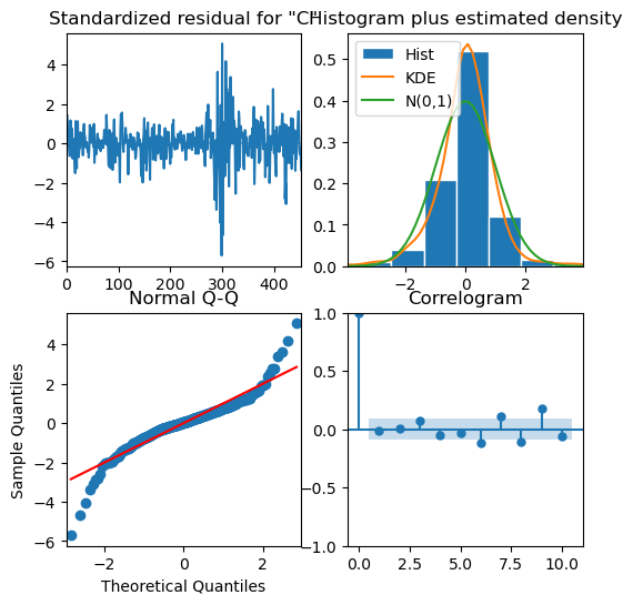
# inspect residuals
modelMA.plot_diagnostics(figsize=(6,6))
plt.show()
# use 95% confidence interval from above to return price forcasts and confidence intervals
pf=[]
pf.append(price_train[-1])
confd = []
confd.append(price_train[-1])
confu = []
confu.append(price_train[-1])

for ret,dn,up in zip(forecast.predicted_mean.values,conf_int95['lower Close'].values,conf_int95['upper Close'].values):
    new_price = price_train[-1] * (1 + ret)
    confu.append(price_train[-1] * (1 + up))
    confd.append(price_train[-1] * (1 + dn))

    pf.append(new_price)

fig,ax = plt.subplots()
ax.plot(price_train.index,price_train.values,color='b',label='Price Train')
ax.plot(price_test.index,price_test.values,color='r',label='Price Test')
ax.plot(price_test.index,pf,color='k',label='Forecast')
ax.fill_between(price_test.index,confd,confu,alpha=0.2,color='b',label='95% CI')
ax.set_title(f'Predicted Stock Price-{ticker} using AR')
ax.legend()
plt.gcf().autofmt_xdate()

AR(1) model does a similar job to MA(1) at predicting the stock trend but still is not able to predict it to good affect. Both models are similar to trivial model with last price forcasting.
ARIMA Models
ARIMA models are a combination of three key components: AutoRegressive (AR), Integrated (I), and Moving Average (MA). The advantage of intergration parameter is that is non-stationary data is used it can make it stationary by defining the integration parameter.
Three parameters are to be defined p (dicussed above for AR), q (dicussed for MA) and d (control for level difference). d=1 is makes the model ARMA which is a limiting case of ARIMA (p,1,q) models but is also a good model given by:
\[Xt = \alpha_1 dX_{t−1} + \alpha_2 dX_{t−2} ... + \alpha_p dX_{t−p} + \epsilon_t + \beta_1 d\epsilon_{t−1} + \beta_2 d\epsilon_{t−2} ... + \beta_q d\epsilon_{t−q}\]Pros
- ARIMA allows us to work with raw data without considering if it is stationary.
- It performs well with high-frequent data. It is less sensitive to the fluctuation in the data compared to other models.
Cons
- ARIMA might fail in capturing seasonality.
- It work better with a long series and short-term (daily, hourly) data.
- As no automatic updating occurs in ARIMA, no structural break during the analysis period should be observed.
- Having no adjustment in the ARIMA process leads to instability.
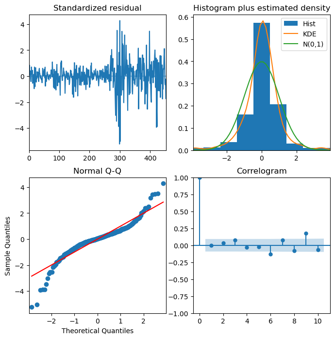
Choosing the parameters from for the ARIMA model. I choose the range 0-10 for the p and q and 0-3 for d. Selection of the parameters for the model is made using Akaike Information Criterion (AIC). The parameters resulting in minimum value of AIC are selected.
\[AIC=2k−2ln(L)\]Where:
- AIC is the Akaike Information Criterion.
- k is the number of parameters in the model.
- ln(L) is the natural logarithm of the likelihood of the model.
stat_test = adfuller(returns.dropna())[0:2]
print(f"The test statistic and p-value of ADF test are {stat_test}")
if stat_test[1] < 0.05:
    print("The returns are stationary")
else:
    print("The returns are not stationary")
The test statistic and p-value of ADF test are (-7.212097179922102, 2.2211435488651752e-10)
The returns are stationary
Since returns are stationary so set d=1
from pmdarima import auto_arima
import warnings
warnings.filterwarnings("ignore")


model = auto_arima(price_train, start_p=0, start_q=0,
            test='adf',
            max_p=12, max_q=12,
            d=1,
            seasonal=True,
            start_P=0,
            D=1,
            trace=True,
            error_action='ignore',
            suppress_warnings=True,
            stepwise=True)
Performing stepwise search to minimize aic
 ARIMA(0,1,0)(0,0,0)[0] intercept   : AIC=2443.312, Time=0.03 sec
 ARIMA(1,1,0)(0,0,0)[0] intercept   : AIC=2385.968, Time=0.21 sec
 ARIMA(0,1,1)(0,0,0)[0] intercept   : AIC=2394.636, Time=0.13 sec
 ARIMA(0,1,0)(0,0,0)[0]             : AIC=2443.519, Time=0.03 sec
 ARIMA(2,1,0)(0,0,0)[0] intercept   : AIC=2387.962, Time=0.14 sec
 ARIMA(1,1,1)(0,0,0)[0] intercept   : AIC=2387.964, Time=0.12 sec
 ARIMA(2,1,1)(0,0,0)[0] intercept   : AIC=2389.416, Time=0.62 sec
 ARIMA(1,1,0)(0,0,0)[0]             : AIC=2388.723, Time=0.03 sec

Best model:  ARIMA(1,1,0)(0,0,0)[0] intercept
Total fit time: 1.302 seconds
# inspect residuals
model.plot_diagnostics(figsize=(8,8))
plt.show()
y_forec95, conf_int95  = model.predict(len(price_test),return_conf_int=True,alpha=0.05)
y_forec80, conf_int80  = model.predict(len(price_test),return_conf_int=True,alpha=0.2)
fig,ax = plt.subplots()
ax.plot(price_train.index,price_train.values,color='b',label='Price Train')
ax.plot(price_test.index,price_test.values,color='r',label='Price Test')
ax.plot(price_test.index,y_forec95,color='k',label='Forecast')
ax.fill_between(price_test.index,conf_int95[:,0],conf_int95[:,1],alpha=0.2,color='b',label='95% CI')
ax.fill_between(price_test.index,conf_int80[:,0],conf_int80[:,1],alpha=0.5,color='darkblue',label='80% CI')
ax.set_title(f'Predicted Stock Price-{ticker} using ARIMA')
ax.legend(loc=2)
plt.gcf().autofmt_xdate()
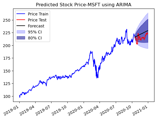
The ARIMA model is able to get capture the trend of the price movement and does a better job at predicting prices. The prices lie within the 80% confidence interval.
Prophet
from prophet import Prophet

alldat = stocks.to_frame().reset_index()
alldat.rename(columns={'Date':'ds','Close':'y'},inplace=True)

# # Specify the split date
# split_date = pd.to_datetime('2020-10-01')

# Split the DataFrame into two based on the split date
train_df = alldat[alldat['ds'] < split_date]
test_df = alldat[alldat['ds'] >= split_date]


m = Prophet(daily_seasonality = True) # the Prophet class (model)
m.fit(train_df)
19:49:16 - cmdstanpy - INFO - Chain [1] start processing
19:49:16 - cmdstanpy - INFO - Chain [1] done processing


<prophet.forecaster.Prophet at 0x14743a500b90>
future = m.make_future_dataframe(periods=64) #we need to specify the number of days in future

fig,ax = plt.subplots()
prediction = m.predict(future)
m.plot(prediction,ax=ax)
ax.set_title(f"Prediction of the {ticker} Stock Price using the Prophet")
ax.set_xlabel("Date")
ax.set_ylabel("Close Stock Price")
ax.plot(test_df['ds'],test_df['y'],color='r')
plt.gcf().autofmt_xdate()
plt.show()
m.plot_components(prediction)
plt.show()
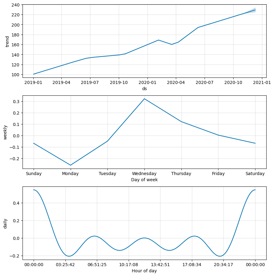
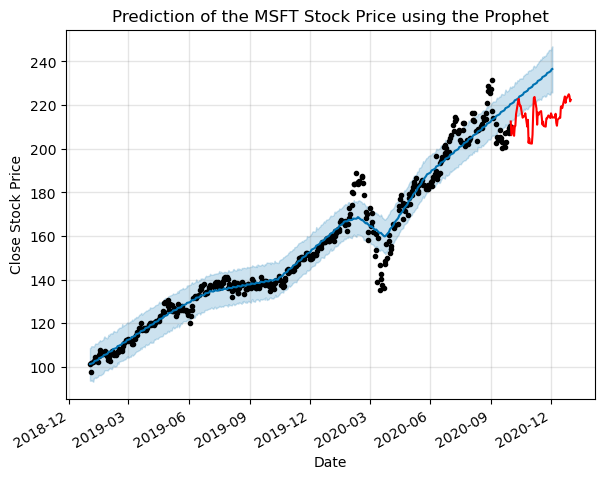
Prophet does not seem to do a good job for predicting the stock future movements out of the box
